监督学习:线性回归与逻辑回归(Supervised Machine Learning: Regression and Classification)
1 机器学习绪论
1.1 what is machine learning
机器学习的定义:field of study that gives computers the ability to learn without being explicitly programmed 在没有明确编程的情况下学习
目前常用的两种机器学习算法:
- 监督学习(Supervised learning)
- 无监督学习(Supervised learning)
Reinforcement learning 强化学习,是另一种机器学习
1.2 监督学习(Supervised learning)
FIGURE:learn from given “right answer”
input(x) $\rightarrow$ output label(y)
最终接受只有输入没有输出(“right answer”),给出合理预测
- 回归算法(regression algorithms),例如根据房价预测;回归试图预测无限多可能的数字中的任意一个
-
分类算法(classification algorithms),例如breast cancer detection 恶性的肿瘤malignant,还是良性的benign;分类只有n种可能的输出,predict categories,是猫还是狗.需要找到分类的边界
案例:given email labeled as spam/not spam,learn a spam filter
1.3 无监督学习(Unsupervised learning)
定义:data only comes with inputs x, but not output labels y
Algorithm has to find structure in the data
给定的数据与任何输出标签y无关,我们的工作是找到一些结构或者模式,或者只是在数据中找到有趣的东西
- 类聚算法(clustering algorithm),将未标记的数据放入不同的集群中;在没有监督的情况下寻找分类,group similar data points together.
- 案例1:given a set of news articles found on the web,group them into sets of articles about the same story.熊猫的新闻中出现了panda,zoo,japan等等词,类聚算法会将他们自动查找并归类;一天有很多新闻,算法可以无监督地寻找归类cluster。
- 案例2:given a database of customer data,automatically discover market segments and group customers into different market segments
-
异常检测(Anomaly detection):find unusual data points
- 降维(Dimensionality reduction):将大数据集压缩维小数据集同时尽可能丢失少的信息
1.4 Jupiter notebook
运行代码:按住 Shift 键并按 ‘Enter’
2 单变量线性回归
| 单词 | 释义 | 单词 | 释义 |
|---|---|---|---|
| hypothesis | 假设函数 | Linear regression | 线性回归 |
| Parameter | 模型参数 | cost function | 代价函数 |
| Gradient descent | 梯度下降 | convex function | 凸函数 |
2.1 线性回归模型(Linear Regression Model)
数据集被称作训练集(data set)
Notation:
- m = Number of training examples →训练样本的数量
- x’s = “input” variable / features →输入变量 / 特征
- y’s = “output” variable / “target” variable →输出变量 / 目标变量
- (x, y) = single training example →一个训练样本
- ($ x^{(i)}$,$ y^{(i)}$) = ith training example →第i个训练样本
2.2 Cost function 成本/损失函数
Model模型:$ f_{\mathbf{w},b}(\mathbf{x}^{(i)}) = \mathbf{w} \cdot \mathbf{x}^{(i)} + b $
Parameter参数: $\mathbf{w},\mathbf{X}$
Cost function成本函数:
$J(\mathbf{w},b) = \frac{1}{2m} \sum\limits_{i = 0}^{m-1} (f_{\mathbf{w},b}(\mathbf{x}^{(i)}) - y^{(i)})^2 $
Objective目标: 使成本函数$J(\mathbf{w},b)$最小
2.3 Gradient descent 梯度下降
2.3.1 什么是梯度算法
梯度下降是用来找到$J(\mathbf{w},b)$最小值的算法
- 随机从$w$和$b$的某个值出发
- 一步一步下山直至收敛到局部最低点
- 梯度下降算法的特点:不同的起始点出发会到达不同的局部最小值(local minima)
2.3.2 梯度算法表达式
下面我们来实现梯度下降(Gradient descent)的算法
多个变量的梯度算法:(重复执行直到满足收敛条件为止)
\[\begin{aligned} \text{repeat}&\text{ until convergence:} \; \lbrace \newline\; & w_j = w_j - \alpha \frac{\partial J(\mathbf{w},b)}{\partial w_j} \; & \text{for j = 0..n-1}\newline &b\ \ = b - \alpha \frac{\partial J(\mathbf{w},b)}{\partial b} \newline \rbrace \end{aligned}\]在这个等式中,$\alpha$是学习率(learning rate),通常是0~1之间的小正数。如果$\alpha$非常大,说明正在采取非常激进的下坡方式,每一步迈得很大。
事实上,学习率不能过小或过大。
- 如果学习率过小,每一步都很小,程序会很慢
- 如果学习率过大,程序一步就会迈过极小值,会越来越发散
2.3.3 Simultaneous update 同步更新
正确的更新方式:
\[\begin{aligned} & temp_w = w_j - \alpha \frac{\partial J(\mathbf{w},b)}{\partial w_j} \; & \text{for j = 0..n-1}\newline &temp_b \ = b - \alpha \frac{\partial J(\mathbf{w},b)}{\partial b} \newline & w = temp_w \newline & b = temp_b \end{aligned}\]下面这个是错误的更新方式:
\[\begin{align*} & temp_w = w_j - \alpha \frac{\partial J(\mathbf{w},b)}{\partial w_j} \; & \text{for j = 0..n-1}\newline & w = temp_w \newline &temp_b \ = b - \alpha \frac{\partial J(\mathbf{w},b)}{\partial b} \newline & b = temp_b \end{align*}\]- 更新方程时需要同时更新$w$和$b$
- 正确方法:先同时计算右边部分,然后同时更新$w$和$b$
- $\times$错误方法:先计算temp0然后更新θ_0,再计算temp1然后更新θ_1
2.4 Gradient descent for linear regression线性回归中的梯度下降算法
- 线性回归中不会出现多个极小值,三维图像永远是碗形,即convex function
- bashed gradient descent指的是在梯度下降的每一步中,我们都在查看所有的训练事例,使用了整个训练集(因为有求和)
3 Multivariate linear regression 多元线性回归
名词翻译
| 单词 | 词义 | 单词 | 词义 |
|---|---|---|---|
| feature | 特征 | Multivariate linear regression | 多元线性回归 |
| Feature Scaling | 特征缩放 | Example automatic convergence test | 自动收敛测试 |
| Polynomial regression | 多项式回归 | Normal equation | 正规方程 |
3.1 Multiple features 多元线性回归
多元线性回归:即有多个特征的线性回归
- n = number of features →训练样本的数量
- $\overrightarrow{x}^{(i)}$ = input features of ith training example →第i个训练样本的输入特征值,在多元特征中,$\overrightarrow{x}^{(i)}$是一个一维向量,即一行多列
- $x_j^{(i)}$ = value of feature j in ith training example →第i个训练样本中第j个特征值
3.2 多元线性回归的梯度下降
3.2.1 常规解法
\[\begin{align*}\text{Parameters }&\overrightarrow{w} = [w_1 \ w_2 \ ...\ w_n] \newline &b\text{ \ still a number} \newline \text{model }& f_{\overrightarrow{w},b}(\mathbf{x})=\overrightarrow{w}\cdot\overrightarrow{x}+b \newline \text{cost function \ } &J(\overrightarrow{w},b) = \frac{1}{2m} \sum\limits_{i = 0}^{m-1} (f_{\overrightarrow{w},b}(\mathbf{x}^{(i)}) - y^{(i)})^2 \newline \text{Gradient decent }& w_j = w_j - \alpha \frac{\partial J(\overrightarrow{w},b)}{\partial w_j} \; \text{for j = 0..n-1} \newline & b = b - \alpha \frac{\partial J(\overrightarrow{w},b)}{\partial b} \end{align*}\]3.2.2 Normal equation 正规方程 (只适用于线性回归)
- 提供了一个求最小值的解析解法
- 正规方程不需要学习率,不用迭代
- 正规方程速度较慢
3.3 Feature Scalling 特征缩放
3.3.1 特征缩放可以使梯度更快收敛
当一个案例有不同的特征,他们具有不同的值的范围,会导致梯度下降运行缓慢
例如,在房价预测中,房间面积$x_1$为2000,房间数量$x_2$为5,最终价格300k 参数$w_1=0.05$,参数$w_2=50$,参数$b=50$,等高线是椭圆,做梯度下降会运行缓慢 假如对$x_1 ,x_2$做缩放,使得范围相近,等高线变为圆形,加快梯度下降
因此,我们需要特征缩放,来使得特征调整到相似的尺度范围
3.3.2 Mean normalization 均值归一化
方法1.除以最大值
$x_1$在区间[a,b]中,$x_2$在区间[c,d]中
归一化后,$\widehat{x_1}=\frac{x_1}{b}$,$\widehat{x_2}=\frac{x_2}{b}$
方法2. Mean normalization
$x_1$在区间[a,b]中,$x_2$在区间[c,d]中
计算得到$x_1$的平均值$\mu_1$,$x_2$的平均值$\mu_2$
归一化后,$\widehat{x_1}=\frac{x_1-\mu_1}{b-a}$,$\widehat{x_2}=\frac{x_2-\mu_2}{d-c}$
此时$\widehat{x_1}$和$\widehat{x_2}$在(-1,1)内部
方法3. Z-score normalization Z分数归一化
求出平均值$\mu_1$和标准差(standard deviation)$\sigma_1$
归一化后,\(\widehat{x^{(i)}_j} = \dfrac{x^{(i)}_j - \mu_j}{\sigma_j}\)
其中, \(\begin{align*} \mu_j &= \frac{1}{m} \sum_{i=0}^{m-1} x^{(i)}_j \newline \sigma^2_j &= \frac{1}{m} \sum_{i=0}^{m-1} (x^{(i)}_j - \mu_j)^2 \end{align*}\)
注意${x^{(i)}_j}$表示第i个训练样本的第j个特征
在z分数归一化后,所有要素的平均值为0,标准差为1
3.4 检查梯度下降是否收敛
方法一:画一张图
方法二:Automatic convergence test
令$\epsilon = 10^{-3}$
如果在一次迭代中,$J(\overrightarrow{w},b) \leq \epsilon$
那么可以认为收敛
3.5 选择合适的学习率
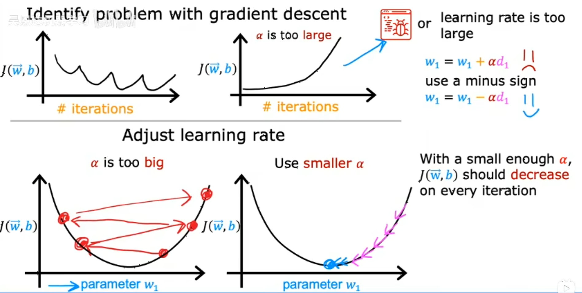
一个debug小技巧,把$\alpha$设置的很小,来检查成本函数是否会下降
如果此时成本函数仍然上升,说明程序中有bug
反复尝试0.001,0.01,0.1,1等数值,选择下降较快的学习率
3.6 Feature Engineering 特征工程
可以根据现实情况,组合原本的特征
例如在房价预测中,地块长度$x_1$,宽度$x_2$,原本的函数为 \(f_{\overrightarrow{w},b}=w_1x_1+w_2x_2+b\) 然而我们知道地块面积$x_3=x_1x_2$也与房价有关,函数变为 \(f_{\overrightarrow{w},b}=w_1x_1+w_2x_2+w_3x_3+b\) 这就是特征工程
特征工程主要包括
- 特征选择:从众多特征中选择出最具代表性和区分性的特征,以减少特征维度,提高模型效率和泛化能力。常见的方法有过滤法(如方差分析、相关系数法)、包装法(如递归特征消除法)和嵌入法(如基于 L1 正则化的特征选择)。
- 特征构建:结合领域知识,通过对现有特征进行组合、变换等操作,创建新的特征。例如,在电商数据分析中,可以根据用户的购买时间和购买金额构建平均购买单价、购买频率等新特征。
3.7 多项式回归(Polynomial regression)
3.7.1 多项式回归的概念
多项式回归是线性回归的扩展,通过增加自变量的高次项来拟合数据,能处理非线性关系。模型形式为 $y = \theta_0 + \theta_1x + \theta_2x^2 + \cdots + \theta_nx^n$
- 实质是将原始特征 $x$ 转换为包含高次项的特征矩阵 $[x, x^2, \cdots, x^n]$。
- 能拟合复杂的非线性关系,灵活性高。
- 容易过拟合,尤其当多项式次数过高时。
3.7.2 代码实例
import numpy as np
from sklearn.preprocessing import PolynomialFeatures
from sklearn.linear_model import LinearRegression
from sklearn.metrics import mean_squared_error, r2_score
from sklearn.model_selection import train_test_split

# 生成示例数据
np.random.seed(0)
X = np.sort(5 * np.random.rand(80, 1), axis=0)
y = np.sin(X).ravel() + np.random.randn(80) * 0.1

# 划分训练集和测试集
X_train, X_test, y_train, y_test = train_test_split(X, y, test_size=0.2, random_state=42)

# 多项式特征转换,使用PolynomialFeatures将原始特征转换为多项式特征
degree = 3  # 多项式次数
poly = PolynomialFeatures(degree=degree)
X_train_poly = poly.fit_transform(X_train)
X_test_poly = poly.transform(X_test)

# 线性回归拟合
model = LinearRegression()
model.fit(X_train_poly, y_train)

# 预测
y_pred = model.predict(X_test_poly)

# 评估模型,使用 mean_squared_error 和 r2_score 评估模型性能
mse = mean_squared_error(y_test, y_pred)
r2 = r2_score(y_test, y_pred)
print(f"均方误差 (MSE): {mse}")
print(f"决定系数 (R^2): {r2}")
3.8 利用Scikit-Learn进行回归
3.8.1 线性回归模型(LinearRegression)
# 导入numpy库和sklearn库
import numpy as np
from sklearn.linear_model import LinearRegression

# 导入数据
X_train = np.array([[1], [2], [3], [4], [5]])
y_train = np.array([2, 4, 6, 8, 10])

# 创建并训练线性回归模型
model = LinearRegression()
model.fit(X_train, y_train)

# 待预测的数据
X_test = np.array([[6], [7]])

# 使用predict函数进行预测
y_pred = model.predict(X_test)
print("预测结果:", y_pred)
3.8.2 逻辑回归模型(LogisticRegression)
import numpy as np
from sklearn.linear_model import LogisticRegression

# 训练数据
X_train = np.array([[1], [2], [3], [4], [5]])
y_train = np.array([0, 0, 1, 1, 1])

# 创建并训练逻辑回归模型
model = LogisticRegression()
model.fit(X_train, y_train)

# 待预测的数据
X_test = np.array([[6], [7]])

# 进行预测
y_pred = model.predict(X_test)
print("预测结果:", y_pred)
3.8.3 决策树模型(DecisionTreeClassifier)
import numpy as np
from sklearn.tree import DecisionTreeClassifier

# 训练数据
X_train = np.array([[1], [2], [3], [4], [5]])
y_train = np.array([0, 0, 1, 1, 1])

# 创建并训练决策树分类器
model = DecisionTreeClassifier()
model.fit(X_train, y_train)

# 待预测的数据
X_test = np.array([[6], [7]])

# 进行预测
y_pred = model.predict(X_test)
print("预测结果:", y_pred)